HBOMS epi model example

In this notebook, we show a simple SEIR-model example with multiple units. These units might correspond to different communities in which a pathogen spreads, isolated by space (or time, or otherwise).

We first have to import the hboms package, which provides the building blocks for defining a model. We also import some utilities (for displaying stan models with syntax highlighting), and some other python modules for statistics and plotting.

import hboms
import hboms.utilities as util
import matplotlib.pyplot as plt
import numpy as np
import scipy.stats as sts

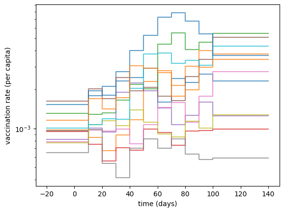
Vaccination data

Here I assume that the vaccination data can be transformed in a per-capita vaccination rate. This rate is modeled as a smoothed, piece-wise constant function, with levels that are unit-specific, but with change points (knots) that are the same for all units.

The smoothed rate function is given by

\[ \eta(t) = \sum_{i=1}^{n-1} \eta_i \mathrm{expit}(t - \tau_i) [1 - \mathrm{expit}(t - \tau_{i+1})] \]

where \(n\) is the number of knots. This is slightly inefficient, as for \(t\) far away from \(\tau_i\) and \(\tau_{i+1}\) the expit terms are practically zero.

We set the first and last knot \(\tau_1\) and \(\tau_n\) to values way beyond the observed interval. Notice that outside the interval \([\tau_1, \tau_n]\), the vaccination rate is very close to zero. For this example, the time interval is going to be \(t \in [0, 120]\) days, and we choose \(\tau_1 = -20\) and \(\tau_n = 140\).

## vaccination rates 

R = 12 # number of units
knots = np.array([-20] + [10*i for i in range(1,11)] + [140])
num_knots = len(knots)

vacc_rates = [
    0.001 * np.exp(np.cumsum(sts.norm.rvs(size=num_knots-1, loc=0.1, scale=0.3)))
    for _ in range(R)
]

fig, ax = plt.subplots(1, 1)

for vr in vacc_rates:
    vre = list(vr) + [vr[-1]]
    ax.step(knots, vre, where='post', alpha=0.7)

ax.set_yscale('log')
ax.set_xlabel("time (days)")
ax.set_ylabel("vaccination rate (per capita)")

Text(0, 0.5, 'vaccination rate (per capita)')

Define an HBOMS model

Every HBOMS model has the following obligatory components:

• a list of parameters. A parameter has to be defined with the Parameter class from the hboms module. The Parameter class has 3 required arguments: name, value and type. The name must be unique, the value is the initial guess and the type determines if the parameter is a constant, fixed between units, or varies between units.

• A list of state variables. Use Variable objects from the hboms module to create these state variables. It is possible to define vector-valued state variables, but this is still experimental. This should make it easy to define e.g. age classes in epi models.

• A string defing the ODE model. This is regular Stan code, and can contain any Stan expression or statement. The ODE model will have access to all the unit-specific or shared parameters used in this piece of code. At this point, non-constant parameters have to be scalars. Constants are allowed to be vectors or matrices. In addition to parameters, the ODE function has access to the state variables by name. For each state variable X, a variable ddt_X is declared, and the user is supposed to define these time derivatives.

• A string defining the initial condition. The user has automatic access to the parameters, and for each state variable X, an initial value X_0 is declared, which the user must define.

• A list of distributions defining the model likelihood. Distributions are defined using the StanDist class, which takes the name of a Stan distribution as its first argument, then the name of the observation and then a list of parameters. The parameters can be arbitrary Stan expressions.

• Finally, a list of observations must be given. Use Observation from the hboms module to create these. The data type (in this case an integer) must be specified, as the default is a real number.

In addition to these, we can also specify optional components. In our case

• trans_state, which is a list of additional state variables, which can be computed from the ODE state variables.

• transform a string with Stan statements specifying how to compute the transformed state variables.

• options is a python dict with some integration options. It specifies the ODE integrator tolerance parameters etc. The option unit_obs is a boolean which must be set to True is you have any observations at time t=0. This is because Stan by default does not allow evaluation of the ODEs at t=0, and we add some code to circumvent this.

Some things to avoid:

• Don’t use the names R, r, N, n, u_sim state. It’s probably a bad idea to start variables with ddt_ or end them with _0 or _sim. There are currently no warnings when you violate these rules.

We can choose from the following parameter types. The “H” in HBOMS is currently only justified by the random parameter.

• random: random-effects like parameter. Normal or log-Normal distribution with estimated location and scale parameters.

• fixed: parameter shared between all units.

• indiv: Different parameter for each unit. Location and scale not estimated.

• const: A constant shared by all units

• const_indiv: A constant that is different for all units.

The space in which a parameter lives can be

• real: this is the default and valid for all parameters

• vector: Currently only implemented for const and const_indiv parameters. The dimension of the vector space must be the same for each unit. So you might have to add some padding.

• matrix The same restrictions hold as for vector.

# parameters are positive by default. set lbound=None to avoid this.
params = [
    hboms.Parameter("R0m1", 0.5, "random", scale=0.15), # R_0 - 1
    hboms.Parameter("alpha", 0.5, "const"), # rate E -> I
    hboms.Parameter("gamma", 0.4, "random", scale=0.1), # recovery rate
    hboms.Parameter("theta", 300, "const"), # scale to population size
    hboms.Parameter("epsilon", 1e-4, "const"), # inoculum size
    hboms.Parameter("phi", 1e3, "fixed"), # overdispersion parameter
    hboms.Parameter("eta", vacc_rates, "const_indiv", space="vector"), # per-capita vaccination rate
    hboms.Parameter("tau", knots, "const", lbound=None, space="vector"), # vacc-rate change points
]

# the variable V is the cumulative fraction of vaccinated individuals
state = [
    hboms.Variable("S"), 
    hboms.Variable("E"), 
    hboms.Variable("I"), 
    hboms.Variable("V")
]

# beta and gamma are correlated. Does it help to reparameterize with R0m1 = beta / gamma - 1?
odes = """
real beta = gamma * (R0m1 + 1);
int n = num_elements(tau);
real vacc_rate = sum(eta .* inv_logit(t - tau[1:n-1]) .* inv_logit(tau[2:n] - t));
ddt_S = -beta * S * I - vacc_rate * S;
ddt_E = beta * S * I - alpha * E;
ddt_I = alpha * E - gamma * I;
ddt_V = vacc_rate * S;
"""

# We define C = theta * I, which is the expected number of cases.
trans_state = [hboms.Variable("C")]

transform = """
C = theta * I;
"""

init = """
S_0 = 1.0 - epsilon;
E_0 = 0.0;
I_0 = epsilon;
V_0 = 0.0;
"""

obs = [
    hboms.Observation(name="Cases", data_type="int")
]

dists = [
    hboms.StanDist(
        name="neg_binomial_2", 
        obs_name="Cases", 
        params=["C", "phi"]
    )
]


options = {
    "integrator" : "ode_rk45_tol",
    "rel_tol": 1e-9,
    "abs_tol": 1e-9,
    "max_num_steps": 100000
}

# define and compile the HBOMS model

hbm = hboms.HbomsModel(
    name="seir_model",
    state=state,
    odes=odes,
    init=init,
    params=params,
    obs=obs,
    dists=dists,
    trans_state=trans_state,
    transform=transform,
)

10:57:36 - cmdstanpy - INFO - compiling stan file /home/chris/Repositories/hboms/notebooks/seir_model.stan to exe file /home/chris/Repositories/hboms/notebooks/seir_model
10:58:06 - cmdstanpy - INFO - compiled model executable: /home/chris/Repositories/hboms/notebooks/seir_model

Have a look at the Stan model in full color.

util.show_stan_model(hbm.model_code)

functions {
    /* vector field */
    vector ode_fun(real t, vector state, real R0m1, data real alpha, real gamma, data vector eta, data vector tau) {
        /* unpack the state variables */
        real S = state[1];
        real E = state[2];
        real I = state[3];
        real V = state[4];
        /* declare derivatives of state variables */
        real ddt_S, ddt_E, ddt_I, ddt_V;
        /* user-defined ODEs */
        real beta = gamma * (R0m1 + 1);
        int n = num_elements(tau);
        real vacc_rate = sum(eta .* inv_logit(t - tau[1:n-1]) .* inv_logit(tau[2:n] - t));
        ddt_S = -beta * S * I - vacc_rate * S;
        ddt_E = beta * S * I - alpha * E;
        ddt_I = alpha * E - gamma * I;
        ddt_V = vacc_rate * S;
        /* return literal vector with derivatives */
        return [ddt_S, ddt_E, ddt_I, ddt_V]';
    }
    /* initial condition */
    vector gen_init(data real epsilon) {
        /* declare initial variables */
        real S_0, E_0, I_0, V_0;
        /* user-defined initial condition */
        S_0 = 1.0 - epsilon;
        E_0 = 0.0;
        I_0 = epsilon;
        V_0 = 0.0;
        /* return literal vector with initival state variables */
        return [S_0, E_0, I_0, V_0]';
    }
    /* state transform function */
    vector state_transform(real t, vector state, data real theta) {
        /* unpack required state variables */
        real I = state[3];
        /* declare transformed state variables */
        real C;
        /* user-defined transformation code */
        C = theta * I;
        /* return literal vector with transformed variables */
        return [C]';
    }
    /* IVP solver function */
    array[] vector solve_ivp(data array[] real Time, real R0m1, data real alpha, real gamma, data real theta, data real epsilon, data vector eta, data vector tau) {
        int N = num_elements(Time); /* number of time points */
        vector[4] init_state = gen_init(epsilon); /* generate initial state */
        array[N] vector[5] sol; /* allocate space for solution */
        sol[1:N, 1:4] = ode_rk45(ode_fun, init_state, 0.0, Time[1:N], R0m1, alpha, gamma, eta, tau); /* solve initial value problem */
        for ( n in 1:N ) sol[n, 5:5] = state_transform(Time[n], sol[n, 1:4], theta); /* compute transformation of the state and append to the trajectory */
        return sol; /* and return the result */
    }
    /* auxiliary function for map_rect */
    vector map_rect_helper_fun(vector ppar, vector upar, data array[] real rdat, data array[] int idat) {
        int N = idat[1]; /* number of time points */
        /* find shapes of non-scalar parameters */
        int shape_eta = idat[2];
        int shape_tau = idat[3];
        /* solve initial value problem */
        array[N] vector[5] sol = solve_ivp(rdat[1 + 3 + shape_eta + shape_tau:N + 3 + shape_eta + shape_tau], upar[1], rdat[1], upar[2], rdat[2], rdat[3], to_vector(rdat[4:3 + shape_eta]), to_vector(rdat[4 + shape_eta:3 + shape_eta + shape_tau]));
        /* concatenate solution into a vector */
        vector[5 * N] res;
        for ( n in 1:N ) res[(n - 1) * 5 + 1:n * 5] = sol[n];
        return res;
    }
    /* log-likelihood function */
    vector loglik_fun(int Cases, vector state, real phi) {
        /* unpack required state variables */
        real C = state[5];
        /* declare log-lik variables */
        real ll_Cases = 0.0;
        /* user-defined log-likelihood */
        ll_Cases = neg_binomial_2_lpmf(Cases | C, phi); /* neg_binomial_2 log-likelihood */
        return [ll_Cases]';
    }
    /* rng function */
    int Cases_rng(vector state, real phi) {
        /* unpack required state variables */
        real C = state[5];
        /* declare variable to-be-returned */
        int Cases;
        /* user-defined sampler */
        Cases = neg_binomial_2_rng(C, phi); /* random neg_binomial_2 sample */
        return Cases;
    }
}

data {
    int<lower=0> R; /* number of units */
    array[R] int<lower=0> N; /* number of observations per unit */
    array[R, max(N)] real<lower=0.0> Time; /* observation times */
    /* observations */
    array[R, max(N)] int Cases;
    int<lower=0> NSim; /* number of simulation time points */
    array[R, NSim] real<lower=0.0> TimeSim; /* simulation time points */
    /* constants */
    real<lower=0.0> alpha;
    real<lower=0.0> theta;
    real<lower=0.0> epsilon;
    int shape_eta;
    array[R] vector<lower=0.0>[shape_eta] eta;
    int shape_tau;
    vector[shape_tau] tau;
}

transformed data {
    /* declarations */
    array[R, max(N) + 3 + shape_eta + shape_tau] real rdats;
    array[R, 3] int idats; /* integer data */
    /* definitions */
    rdats[:, 1 + 3 + shape_eta + shape_tau:max(N) + 3 + shape_eta + shape_tau] = Time;
    idats[:, 1] = N;
    /* add constants to rdats */
    rdats[:, 1] = rep_array(alpha, R);
    rdats[:, 2] = rep_array(theta, R);
    rdats[:, 3] = rep_array(epsilon, R);
    for ( r in 1:R ) rdats[r, 4:3 + shape_eta] = to_array_1d(eta[r]);
    rdats[:, 4 + shape_eta:3 + shape_eta + shape_tau] = rep_array(to_array_1d(tau), R);
    /* add shapes to idats */
    idats[:, 2] = rep_array(shape_eta, R);
    idats[:, 3] = rep_array(shape_tau, R);
}

parameters {
    /* individual parameters (and their hyper-parameters) */
    array[R] real<lower=0.0> R0m1;
    real loc_R0m1;
    real<lower=0.0> scale_R0m1;
    array[R] real<lower=0.0> gamma;
    real loc_gamma;
    real<lower=0.0> scale_gamma;
    /* fixed parameters */
    real<lower=0.0> phi;
}

transformed parameters {
    array[R] vector[2] upars; /* prepare data structure for map_rect */
    vector[0] ppar; /* no population parameters required for map_rect */
    /* assign unit-parameters to array of vectors */
    upars[:, 1] = R0m1;
    upars[:, 2] = gamma;
}

model {
    /* solve ODEs in parallel */
    vector[sum(N) * 5] concat_res = map_rect(map_rect_helper_fun, ppar, upars, rdats, idats);
    /* compute log-likelihood of observations */
    for ( r in 1:R ) {
        for ( n in 1:N[r] ) {
            /* extract state */
            int idx = 5 * (sum(N[:r - 1]) + n - 1) + 1;
            vector[5] state = concat_res[idx:idx + 4];
            /* compute likelihood of observation given state */
            target += loglik_fun(Cases[r, n], state, phi);
        }
    }
    /* prior */
    R0m1 ~ lognormal(loc_R0m1, scale_R0m1);
    loc_R0m1 ~ student_t(3.0, 0.0, 2.5);
    scale_R0m1 ~ student_t(3.0, 0.0, 2.5);
    gamma ~ lognormal(loc_gamma, scale_gamma);
    loc_gamma ~ student_t(3.0, 0.0, 2.5);
    scale_gamma ~ student_t(3.0, 0.0, 2.5);
    phi ~ student_t(3.0, 0.0, 2.5);
}

generated quantities {
    array[R, NSim] real S_sim, E_sim, I_sim, V_sim, C_sim;
    array[R, max(N)] int Cases_sim;
    vector[sum(N) * 1] log_lik; /* vector of log-likelihoods for model comparison */
    for ( r in 1:R ) {
        array[NSim] vector[5] u_sim = solve_ivp(TimeSim[r], R0m1[r], alpha, gamma[r], theta, epsilon, eta[r], tau); /* solve ODEs at simulation times */
        array[N[r]] vector[5] u_sim_obs = solve_ivp(Time[r, 1:N[r]], R0m1[r], alpha, gamma[r], theta, epsilon, eta[r], tau); /* solve ODEs at observation times */
        for ( n in 1:NSim ) {
            S_sim[r, n] = u_sim[n, 1];
            E_sim[r, n] = u_sim[n, 2];
            I_sim[r, n] = u_sim[n, 3];
            V_sim[r, n] = u_sim[n, 4];
            C_sim[r, n] = u_sim[n, 5];
        }
        for ( n in 1:N[r] ) {
            int idx = 1 * (sum(N[:r - 1]) + n - 1) + 1;
            log_lik[idx:idx + 0] = loglik_fun(Cases[r, n], u_sim_obs[n], phi); /* record log-likelihood of each observation */
            Cases_sim[r, n] = Cases_rng(u_sim_obs[n], phi); /* simulate data at observation times */
        }
    }
}

Use the HBOMS model to simulate some data.

For this, we create and compile a separate Stan model that generates random effects and observations in the generated quantities block. We so have to specify the number of units and time points for each unit. You can add a field “ID” to the data to give each unit a name, which is nice for plots.

The data has to contain the key "Time", with sorted time points for each unit. Integration always starts at time \(t_0 = 0\) (this will be relaxed in the future)

N = [120 for _ in range(R)]

Time = [list(range(1, Nr+1)) for Nr in N]
ID = [f"Epi {i}" for i in range(1, R+1)]

data = {"Time" : Time, "ID" : ID}

sims = hbm.simulate(data, 10) ## 10 simulated data sets
util.show_stan_model(hbm.simulator_code)

10:58:07 - cmdstanpy - INFO - compiling stan file /home/chris/Repositories/hboms/notebooks/seir_model_simulator.stan to exe file /home/chris/Repositories/hboms/notebooks/seir_model_simulator
10:58:28 - cmdstanpy - INFO - compiled model executable: /home/chris/Repositories/hboms/notebooks/seir_model_simulator
10:58:28 - cmdstanpy - INFO - CmdStan start processing
10:58:28 - cmdstanpy - INFO - Chain [1] start processing
10:58:28 - cmdstanpy - INFO - Chain [1] done processing

functions {
    /* vector field */
    vector ode_fun(real t, vector state, real R0m1, data real alpha, real gamma, data vector eta, data vector tau) {
        /* unpack the state variables */
        real S = state[1];
        real E = state[2];
        real I = state[3];
        real V = state[4];
        /* declare derivatives of state variables */
        real ddt_S, ddt_E, ddt_I, ddt_V;
        /* user-defined ODEs */
        real beta = gamma * (R0m1 + 1);
        int n = num_elements(tau);
        real vacc_rate = sum(eta .* inv_logit(t - tau[1:n-1]) .* inv_logit(tau[2:n] - t));
        ddt_S = -beta * S * I - vacc_rate * S;
        ddt_E = beta * S * I - alpha * E;
        ddt_I = alpha * E - gamma * I;
        ddt_V = vacc_rate * S;
        /* return literal vector with derivatives */
        return [ddt_S, ddt_E, ddt_I, ddt_V]';
    }
    /* initial condition */
    vector gen_init(data real epsilon) {
        /* declare initial variables */
        real S_0, E_0, I_0, V_0;
        /* user-defined initial condition */
        S_0 = 1.0 - epsilon;
        E_0 = 0.0;
        I_0 = epsilon;
        V_0 = 0.0;
        /* return literal vector with initival state variables */
        return [S_0, E_0, I_0, V_0]';
    }
    /* state transform function */
    vector state_transform(real t, vector state, data real theta) {
        /* unpack required state variables */
        real I = state[3];
        /* declare transformed state variables */
        real C;
        /* user-defined transformation code */
        C = theta * I;
        /* return literal vector with transformed variables */
        return [C]';
    }
    /* IVP solver function */
    array[] vector solve_ivp(data array[] real Time, real R0m1, data real alpha, real gamma, data real theta, data real epsilon, data vector eta, data vector tau) {
        int N = num_elements(Time); /* number of time points */
        vector[4] init_state = gen_init(epsilon); /* generate initial state */
        array[N] vector[5] sol; /* allocate space for solution */
        sol[1:N, 1:4] = ode_rk45(ode_fun, init_state, 0.0, Time[1:N], R0m1, alpha, gamma, eta, tau); /* solve initial value problem */
        for ( n in 1:N ) sol[n, 5:5] = state_transform(Time[n], sol[n, 1:4], theta); /* compute transformation of the state and append to the trajectory */
        return sol; /* and return the result */
    }
    /* rng function */
    int Cases_rng(vector state, real phi) {
        /* unpack required state variables */
        real C = state[5];
        /* declare variable to-be-returned */
        int Cases;
        /* user-defined sampler */
        Cases = neg_binomial_2_rng(C, phi); /* random neg_binomial_2 sample */
        return Cases;
    }
}

data {
    int<lower=0> R; /* number of units */
    array[R] int<lower=0> N; /* number of observations per unit */
    array[R, max(N)] real<lower=0.0> Time; /* observation times */
    /* non-random parameters and hyper-parameters */
    real loc_R0m1;
    real<lower=0.0> scale_R0m1;
    real<lower=0.0> alpha;
    real loc_gamma;
    real<lower=0.0> scale_gamma;
    real<lower=0.0> theta;
    real<lower=0.0> epsilon;
    real<lower=0.0> phi;
    int shape_eta;
    array[R] vector<lower=0.0>[shape_eta] eta;
    int shape_tau;
    vector[shape_tau] tau;
    /* hyper parameters for correlated parameters */
}

parameters {
    /* no parameters */
}

model {
    /* no model */
}

generated quantities {
    /* random parameter declarations */
    array[R] real<lower=0.0> R0m1;
    array[R] real<lower=0.0> gamma;
    /* simulated observation declarations */
    array[R, max(N)] int Cases;
    /* simulate for each unit */
    for ( r in 1:R ) {
        /* sample random parameters */
        R0m1[r] = lognormal_rng(loc_R0m1, scale_R0m1);
        gamma[r] = lognormal_rng(loc_gamma, scale_gamma);
        /* sample random correlated parameters */
        /* solve initial value problem */
        array[N[r]] vector[5] sol = solve_ivp(Time[r, 1:N[r]], R0m1[r], alpha, gamma[r], theta, epsilon, eta[r], tau);
        for ( n in 1:N[r] ) {
            Cases[r, n] = Cases_rng(sol[n], phi); /* simulate data at observation times */
        }
    }
}

Check intial guesses.

Fitting Bayesian ODE models is (in my experiance) hopeless if you don’t have a reasonable initial parameter guess. I know that is is good practice to start the MCMC from a random state, but with ODEs that just does not work that well.

sim_data, sim_draws = sims[-1] ## pick one of the simulated data sets
state_var_names = ["C"]
fig = hbm.init_check(sim_data, state_var_names=state_var_names, ppd="envelope")

10:58:28 - cmdstanpy - INFO - CmdStan start processing
10:58:28 - cmdstanpy - INFO - Chain [1] start processing
10:58:29 - cmdstanpy - INFO - Chain [1] done processing

Now fit the model

The sample method passes keyword arguments to the sample method from cmdstanpy. It is a good idea to choose a small step_size (which is used as an initial step size for HMC), otherwise you might ruin your carfully chosen initial parameter guess instantly. Increase threads_per_chain to the number of units if you have a large computer.

hbm.sample(
    sim_data, chains=1, threads_per_chain=R,
    step_size=0.01, refresh=1,
    iter_sampling=300, iter_warmup=300
)

10:58:31 - cmdstanpy - INFO - CmdStan start processing

11:00:15 - cmdstanpy - INFO - CmdStan done processing.
11:00:15 - cmdstanpy - WARNING - Non-fatal error during sampling:
Exception: Exception: neg_binomial_2_lpmf: Location parameter is -1.10936e-08, but must be positive finite! (in 'seir_model.stan', line 74, column 8 to column 55) (in 'seir_model.stan', line 155, column 12 to column 58)
Consider re-running with show_console=True if the above output is unclear!

# check out the fits...

fig = hbm.post_pred_check(sim_data, state_var_names=['C'], ppd="envelope")

Look at the parameter estimates

The CmdStanPy fit object can be found in hbm.fit. The method stan_variable extracts the trace of a single parameter, while stan_variables extracts a python dict with all samples. You might explore further statistics with the arviz package. For instance, the generated quantity log_lik contains the log-likelihood of all observations and can be used for model comparison, using arviz.loo and arviz.compare.

The method simulate returns a list of pairs of simulated data sets and the corresponding random parameter draws, both in a dictionary. We can now compare the conditional distribution of the random parameters with the ground-truth values.

R0m1_hats = hbm.fit.stan_variable("R0m1")
gamma_hats = hbm.fit.stan_variable("gamma")

R0m1_gt = sim_draws["R0m1"]
gamma_gt = sim_draws["gamma"]

fig, axs = plt.subplots(2, 1, figsize=(7,5), sharex=True)

pos = list(range(R))
axs[0].violinplot(R0m1_hats + 1, positions=pos)
axs[0].scatter(pos, R0m1_gt + 1, color='r')

axs[1].violinplot(gamma_hats, positions=pos)
axs[1].scatter(pos, gamma_gt, color='r')

axs[1].set_xticks(pos)
axs[1].set_xticklabels(ID, rotation=90)

axs[0].set_ylabel("$R_0$")
axs[1].set_ylabel("$\\gamma$")

Text(0, 0.5, '$\\gamma$')

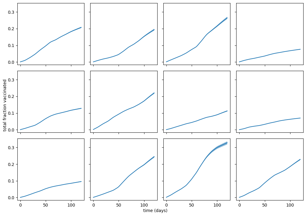
Vaccination coverage

In the posterior predictive checks above, we could also include the variable \(V\), which corresponds to the total fraction of vaccinated individuals. However, \(V \in [0,1]\) and the observed cases are much larger, so we’ll plot \(V\) separately. The variable \(V\) should pretty much correspond to the vaccination data. However, in the model we only vaccinate \(S\)-individuals, and the rate is per-capita, so there might be some discrepancies.

fig, axs = plt.subplots(3, 4, figsize=(10,7), sharex=True, sharey=True)

for r, ax in enumerate(axs.flatten()):
    Vsim = hbm.fit.stan_variable("V_sim")[:,r,...]
    Vsim_mean = np.mean(Vsim, axis=0)
    Vsim_lo, Vsim_hi = np.percentile(Vsim, axis=0, q=[2.5, 97.5])
    tsim = np.linspace(0, 120, Vsim.shape[1])
    ax.plot(tsim, Vsim_mean)
    ax.fill_between(tsim, Vsim_lo, Vsim_hi, alpha=0.5, linewidths=0)
    
fig.tight_layout()

fig.text(0.5, 0, "time (days)", ha='center')
fig.text(0, 0.5, "total fraction vaccinated", rotation=90, va='center')

Text(0, 0.5, 'total fraction vaccinated')